Excel - Merge Tables with Index and Match Formulas

A lot of the times, I find myself having multiple Excel or CSV files with different tables & data that at some point, I need to merge them...

Here is a not to myself! Use Index and Match formulas.

Index Function

The INDEX function returns a value or the reference to a value from within a table or range.

Match Function

The MATCH function searches for a specified item in a range of cells, and then returns the relative position of that item in the range. For example, if the range A1:A3 contains the values 5, 25, and 38, then the formula =MATCH(25,A1:A3,0) returns the number 2, because 25 is the second item in the range.

Ex :

INDEX (return_range, MATCH (lookup_value, lookup_range, 0))


=INDEX(Sheet1!$B$2:$B$218,MATCH($A2,Sheet1!$A$2:$A$218,0))

In this example, with Match, we're trying to find cell A2's exact value by looking in the "Sheet1", from A2 to A218. When the exact value of A2 is found in the range of Sheet1!$A$2:$A$218, with the Index formula, we pull it's value in the Sheet1!$B$2:$B$218 range!


Another nice article that helped me online ;

https://www.ablebits.com/office-addins-blog/2018/10/31/excel-merge-tables-matching-columns/

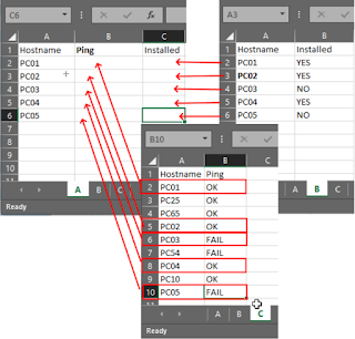
Let’s say, we have an Excel file with 3 sheets. First sheet is named “A”, second “B”, and third “C”. Sheet “A” contains only a list of hostnames. Sheet “B” contains a list of hostnames and a column that indicates if it’s installed or not. Lastly, sheet “B” contains another list of hostnames and their PING results. Sheet “C” contains the same hostnames from the sheet “A” but it has some extra hostnames.

The purpose is to gather all that information about the hostnames found in sheet “A” automatically. Column B of sheet A will bring the PING result from sheet C and Column C of sheet A will bring the “installed” information from sheet B. Perhaps, a picture would be better;

Use the INDEX and MATCH formulas to find the hostnames corresponding in the sheet A from sheet B or C and get their results from the column B to Sheet A. Here is an example;

For Sheet A, Column B2
=INDEX('C'!$B$2:$B$10,MATCH($A2,'C'!$A$2:$A$10))

For sheet A, Column C2
=INDEX(B!$B$2:$B$10,MATCH($A2,B!$A$2:$A$10))